Understanding Oscilloscopes: A Beginner's Guide to Signal Visualization

If you have ever tried debugging a circuit with a multimeter and felt like you were solving a puzzle blindfolded, you are not alone. A multimeter tells you what the voltage is right now. An oscilloscope tells you how it changes over time. That difference is everything.

This guide walks you through what an oscilloscope does, how to read and operate one, which specifications matter, and how to use it in real projects with Arduino, ESP32, and common protocols like I2C and UART.

Why a Multimeter Is Not Enough

A multimeter is indispensable. It measures DC voltage, AC voltage, resistance, continuity, and sometimes capacitance and frequency. But it gives you a single number at a single moment. That is fine for checking a battery voltage or verifying a resistor value.

Now imagine you are generating a PWM signal from an Arduino to control an LED brightness. Your multimeter reads 2.4 V. Is that correct? You have no idea whether the signal is a clean square wave at 490 Hz with a 47% duty cycle, or a noisy mess with ringing and overshoot. You cannot see the shape of the signal.

An oscilloscope draws the voltage on a graph, with time on the horizontal axis and voltage on the vertical axis. It updates this graph continuously, so you can see:

• The exact waveform shape (square, sine, sawtooth, noise)
• Frequency and period
• Duty cycle of PWM signals
• Rise and fall times of digital edges
• Noise, ringing, and glitches
• Communication protocol data (I2C, SPI, UART)
• Timing relationships between multiple signals

If your project involves anything beyond static DC, you need an oscilloscope.

When You Actually Need an Oscilloscope

Here are the real-world situations where a scope becomes essential:

• Debugging PWM signals: Verifying frequency, duty cycle, and clean switching edges for motor drivers, LED dimmers, and servo control.
• Communication protocols: Viewing I2C clock and data lines, UART TX/RX, SPI MOSI/MISO/CLK to diagnose why your sensor is not responding.
• Power supply noise: Measuring ripple voltage on your 3.3 V or 5 V rail to find out why your ADC readings are unstable.
• Timing issues: Checking if two signals are synchronized, measuring propagation delay through a buffer, or verifying that your interrupt handler responds fast enough.
• Analog circuit design: Viewing amplifier output, filter frequency response, oscillator stability.
• Signal integrity: Checking for overshoot, undershoot, and ringing on high-speed digital lines.

Key Specifications Explained

Before buying a scope, understand what the numbers on the spec sheet actually mean.

Specification	What It Means	Recommended Minimum
Bandwidth	The highest frequency the scope can accurately measure (at -3 dB). A 100 MHz scope can reliably show signals up to about 100 MHz.	50 MHz for hobby, 100 MHz for serious work
Sample Rate	How many samples per second the ADC captures. Higher is better for capturing fast edges. Rule of thumb: at least 5x your bandwidth.	500 MSa/s for a 100 MHz scope
Channels	Number of independent inputs. 2 channels lets you compare two signals simultaneously (e.g., clock and data).	2 minimum, 4 is very useful
Memory Depth	How many samples the scope can store in one capture. Deeper memory lets you zoom in on a long capture without losing detail.	1 Mpts minimum
Vertical Resolution	Bits of ADC resolution. Most scopes are 8-bit (256 levels). Higher resolution (10-bit, 12-bit) shows smaller signal details.	8-bit is standard and sufficient for most work
Trigger Types	Edge trigger is basic. Protocol triggers (I2C, SPI, UART) are very helpful for embedded work.	Edge trigger minimum; protocol decode is a strong bonus

The bandwidth rule of thumb: To accurately capture a digital signal, your scope bandwidth should be at least 5x the signal's fundamental frequency. For a 10 MHz clock, use at least a 50 MHz scope. This ensures you can see the edges and not just a rounded approximation.

Types of Oscilloscopes

Analog Oscilloscopes (Obsolete)

These use a cathode ray tube (CRT) to directly deflect an electron beam. They show real-time waveforms with infinite time resolution but cannot store, measure, or analyze signals digitally. You will find them in old labs and on second-hand markets. Not recommended for purchase in 2026.

Digital Storage Oscilloscopes (DSO)

The most common type today. A DSO digitizes the input signal with an ADC, stores it in memory, and displays it on an LCD. This lets you freeze a waveform, zoom in, take automated measurements, save screenshots, and perform math operations like FFT. Every budget scope on the market is a DSO.

Mixed-Signal Oscilloscopes (MSO)

An MSO combines a regular DSO (2 or 4 analog channels) with additional digital input channels (typically 8 or 16). The digital channels work like a logic analyzer, showing high/low states. This is extremely useful for embedded development where you need to see an analog signal alongside a digital bus.

USB Oscilloscopes

These are scope front-ends without a display. They connect to your PC via USB and use software for display and analysis. Advantages: lower cost, large screen, easy data export. Disadvantages: you need a laptop nearby, software can be less responsive than a dedicated scope.

Budget Recommendations for Makers in India

Scope	Bandwidth	Channels	Sample Rate	Approx. Price (INR)	Best For
Hantek DSO5072P	70 MHz	2	1 GSa/s	8,000 - 12,000	Budget entry point
Rigol DS1054Z	50 MHz (hackable to 100 MHz)	4	1 GSa/s	25,000 - 30,000	Best value 4-channel scope
Hantek 6022BE (USB)	20 MHz	2	48 MSa/s	3,500 - 5,000	Absolute budget, basic use
FNIRSI 1014D	100 MHz	2	1 GSa/s	10,000 - 14,000	Portable, tablet-style
Siglent SDS1104X-E	100 MHz	4	1 GSa/s	35,000 - 42,000	Serious hobbyist / professional

The Rigol DS1054Z remains the most recommended first scope in the maker community. Four channels at this price point is rare, and the community firmware hack unlocks all four channels to 100 MHz with protocol decoding. The Hantek DSO5072P is a solid choice if you need two channels on a tight budget.

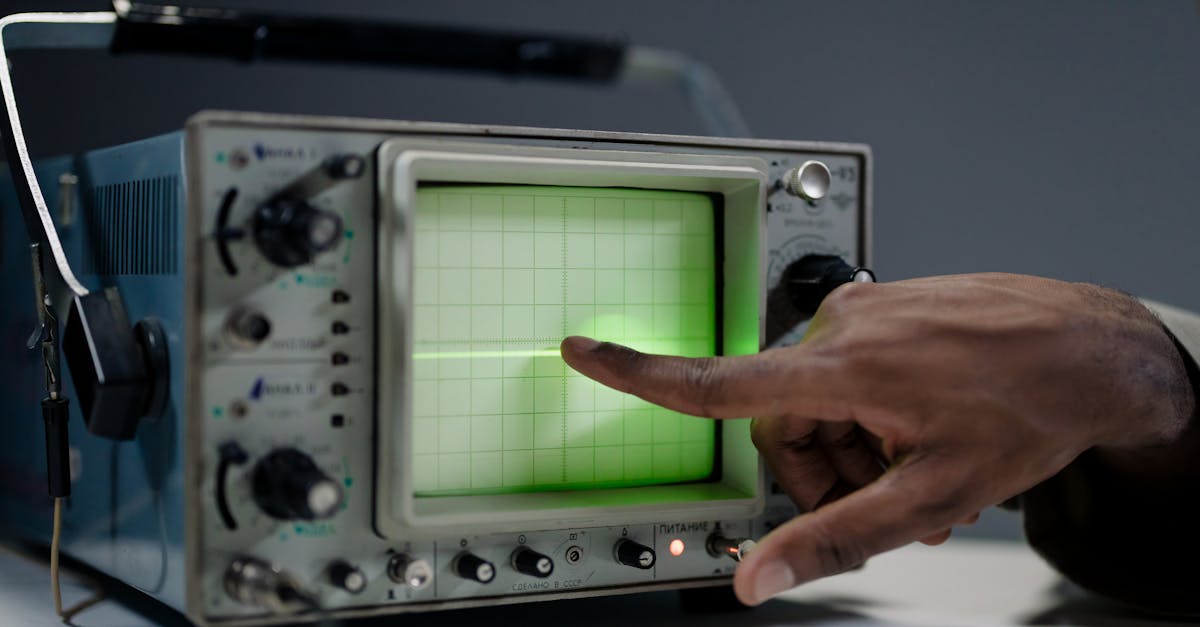
Understanding the Display

An oscilloscope screen is a graph divided into a grid of squares called divisions.

• X-axis (horizontal): Time. Each division represents a fixed time interval, controlled by the time/div knob. If set to 1 ms/div and the screen is 12 divisions wide, you see 12 ms of signal.
• Y-axis (vertical): Voltage. Each division represents a fixed voltage, controlled by the V/div knob. If set to 1 V/div and the screen is 8 divisions tall, the full scale is 8 V.
• Trigger point: Usually marked with an arrow on the right side of the screen. This is the voltage level and edge direction (rising or falling) that tells the scope when to start drawing.
• Ground reference: A small arrow on the left side showing where 0 V is on the screen.

A stable display means the trigger is working correctly. If the waveform is drifting or looks like a jumbled mess, your trigger settings need adjustment.

Essential Controls

Vertical Controls (Per Channel)

• V/div knob: Sets the voltage scale. Turn clockwise to zoom in (fewer volts per division), counter-clockwise to zoom out. Start zoomed out and gradually zoom in.
• Position knob: Moves the waveform up or down on the screen. Useful for separating two channels visually.
• Coupling: DC coupling shows the entire signal including any DC offset. AC coupling blocks the DC component and shows only the AC variation. Use DC coupling by default. Use AC coupling when you want to see small ripple on top of a large DC voltage (like power supply noise on a 5 V rail).

Horizontal Controls

• Time/div knob: Sets the time scale. Turn clockwise to zoom in on time (see fewer microseconds per division), counter-clockwise to zoom out. For a 1 kHz signal, start at about 500 us/div to see a couple of cycles.
• Position knob: Moves the waveform left or right, letting you scroll through captured data.

Trigger Controls

• Level knob: Sets the voltage threshold. The scope starts drawing when the signal crosses this level.
• Slope: Rising edge (most common) or falling edge.
• Source: Which channel to trigger on.

Probe Basics

1X vs 10X Probes

Most oscilloscope probes have a switch with two positions:

• 1X: The probe passes the signal directly. What goes in is what the scope sees. However, the probe adds significant capacitance (around 100 pF) to the circuit, which can distort high-frequency signals.
• 10X: The probe attenuates the signal by a factor of 10 using a built-in voltage divider. The scope compensates by multiplying the displayed value by 10. The advantage is much lower input capacitance (around 10-15 pF) and 10x higher input impedance, causing far less circuit loading.

Use 10X mode by default. Only switch to 1X when measuring very small signals (millivolt range) where you need the extra sensitivity.

Probe Compensation

Every probe has a small trimmer screw or slot near the connector. To compensate:

1. Connect the probe to the scope's calibration output (a square wave, usually 1 kHz at 3.3 V or 5 V, on the front panel).
2. Set the scope to see the square wave clearly.
3. Look at the corners of the square wave:
   • Overshoot (corners have spikes) = overcompensated. Turn the trimmer to reduce.
   • Rounded corners = undercompensated. Turn the trimmer to increase.
   • Clean square corners = properly compensated.

Do this every time you use a new probe or switch between scopes.

Ground Clip

The short wire with an alligator clip is the ground reference. Always connect it to the ground of your circuit. The scope measures voltage between the probe tip and this ground clip. If you do not connect the ground, you will see noise and incorrect readings.

Practical Exercises

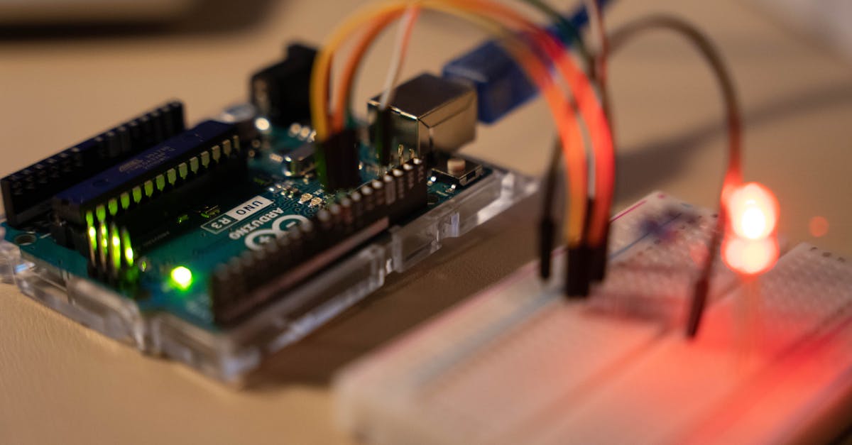
Exercise 1: Viewing Arduino PWM (analogWrite)

Upload this sketch to an Arduino Uno:

void setup() {
  pinMode(9, OUTPUT);
  analogWrite(9, 128); // 50% duty cycle
}
void loop() {}

Scope setup:

1. Connect probe tip to pin 9, ground clip to Arduino GND.
2. Set probe to 10X, scope channel to 10X.
3. Set vertical scale to 2 V/div (signal is 0-5 V, so about 2.5 divisions tall).
4. Set time base to 500 us/div (Arduino PWM is about 490 Hz, so one period is about 2 ms, visible across 4 divisions).
5. Set trigger to rising edge, level at about 2.5 V.

What you should see: A clean square wave. Use the scope's Measure function to read frequency (should be ~490 Hz) and duty cycle (should be ~50%). Try changing analogWrite(9, 64) for 25% duty cycle and observe the change.

Exercise 2: Viewing I2C Communication (ESP32 + Sensor)

Connect an I2C sensor (like a BME280) to an ESP32. Use both scope channels:

• Channel 1: SDA (data line)
• Channel 2: SCL (clock line)

Scope setup:

1. Set both channels to 1 V/div (I2C on ESP32 is 3.3 V logic).
2. Set time base to 20 us/div for 100 kHz standard I2C, or 5 us/div for 400 kHz fast mode.
3. Trigger on Channel 2 (SCL) falling edge.

What you should see: SCL shows a regular clock pattern. SDA changes state between clock pulses. You can identify the start condition (SDA goes low while SCL is high), the address byte, ACK bits, and data bytes. If your scope has I2C protocol decoding, enable it to see the decoded address and data values overlaid on the waveform.

Exercise 3: Viewing UART Serial Data

Send serial data from an Arduino:

void setup() {
  Serial.begin(9600);
}
void loop() {
  Serial.println("Hi");
  delay(1000);
}

Scope setup:

1. Probe the TX pin (pin 1 on Arduino Uno). Ground clip to GND.
2. Set vertical to 2 V/div, time base to 200 us/div for 9600 baud.
3. Trigger on falling edge at about 2.5 V (the start bit pulls the line low).
4. Set trigger mode to Normal (so it waits for the next transmission instead of auto-triggering on noise).

What you should see: Each character appears as a sequence of high and low bits. The start bit (low), 8 data bits (LSB first), and stop bit (high) are visible. The character 'H' is 0x48 in ASCII, which is 01001000 in binary. Reading LSB first from the waveform: 0-0-0-1-0-0-1-0. You can verify this matches.

Exercise 4: Measuring Rise Time

Measuring the rise time of a digital signal tells you about signal integrity and whether your scope has enough bandwidth.

1. Probe any digital output toggling at a known frequency.
2. Zoom in on a rising edge by reducing the time/div to 10-50 ns/div.
3. Use the scope's rise time measurement (usually in the Measure menu), or manually measure the time between 10% and 90% of the signal amplitude.

A typical Arduino digital output has a rise time of about 5-10 ns. If your scope shows a much slower rise time (say 20+ ns), your scope bandwidth may be the limiting factor.

Exercise 5: Finding Power Supply Noise

1. Set your probe to AC coupling (or use the scope's AC coupling setting). This removes the DC component and shows only the variation.
2. Probe your 5 V or 3.3 V power rail. Ground clip to circuit ground.
3. Set vertical scale to 20 mV/div or 50 mV/div.
4. Set time base to 2 us/div for high-frequency switching noise, or 5 ms/div for low-frequency ripple.

What you should see: A good linear regulator output might show less than 10 mV of noise. A cheap switching converter might show 50-100 mV of ripple at its switching frequency (often 500 kHz - 2 MHz). If you see large spikes, those could be causing ADC instability, serial communication errors, or audio noise in your project.

Trigger Modes Explained

Mode	Behavior	When to Use
Auto	Triggers normally when signal is present. If no trigger event occurs within a timeout, it draws anyway.	Default mode. Good for exploring unknown signals or when you just want to see something on screen.
Normal	Only draws when a trigger event occurs. Screen freezes if no trigger.	Use for infrequent or burst signals like UART transmissions, one-shot events, or signals that only appear during specific actions.
Single	Arms once, triggers once, then stops.	Use to capture a one-time event: a power-on glitch, a button press response, a startup sequence. Press the Run/Single button to re-arm.

Tip: If your screen is blank and nothing appears, check if you are in Normal or Single mode. Switch to Auto to see what is happening, then switch back to Normal once you have your trigger dialed in.

Math Functions

FFT (Fast Fourier Transform)

FFT converts your time-domain waveform into a frequency-domain plot, showing which frequencies are present in the signal. This is invaluable for:

• Identifying the switching frequency of a power supply
• Finding clock harmonics causing electromagnetic interference
• Checking if a sine wave oscillator is producing unwanted harmonics
• Measuring the frequency content of audio signals

On most scopes, press the Math button, select FFT, and choose the source channel. Set the center frequency and span to zoom into the region of interest.

Automated Measurements

Modern scopes can automatically measure and display parameters including:

• Frequency and Period
• Duty Cycle (positive and negative)
• Rise Time and Fall Time
• Peak-to-Peak Voltage (Vpp)
• RMS Voltage
• Mean Voltage
• Overshoot and Undershoot (as percentage)
• Phase difference between two channels

Access these through the Measure button. Add the measurements you need and they update in real time. This is far more accurate than counting grid divisions manually.

Common Mistakes to Avoid

1. Ground clip shorting circuits. The ground clip is connected to earth ground through the scope's power cord. If you clip it to a non-ground node in a mains-connected circuit, you create a short circuit. For battery-powered circuits this is rarely an issue, but be extremely careful with anything connected to mains power.

2. Using the wrong coupling mode. If you are in AC coupling and trying to measure a DC voltage, you will read 0 V. If you are in DC coupling trying to see 20 mV of ripple on a 12 V rail, the ripple will be invisible because the vertical scale is too zoomed out. Know which mode you need.

3. Scope bandwidth too low for the signal. A 20 MHz scope cannot accurately show a 16 MHz SPI clock. The waveform will look like a sine wave instead of a square wave, and rise time measurements will be meaningless. Follow the 5x bandwidth rule.

4. Not compensating the probe. An uncompensated probe distorts square wave corners, making your measurements inaccurate. It takes 30 seconds to compensate. Do it.

5. Forgetting to match probe attenuation setting. If your probe is set to 10X but the scope channel is set to 1X, all your voltage readings will be off by a factor of 10. Most modern scopes auto-detect this, but double-check.

6. Using 1X probe mode for high-frequency signals. The added capacitance of 1X mode loads the circuit and rounds off fast edges. Always use 10X for signals above a few hundred kHz.

Oscilloscope vs Logic Analyzer

Feature	Oscilloscope	Logic Analyzer
Shows	Analog waveform shape (voltage over time)	Digital states (high/low over time)
Channels	2-4 analog	8-32+ digital
Best for	Signal quality, analog circuits, rise times, noise, voltage levels	Protocol decoding, timing between many digital signals, state machines
Voltage detail	Full resolution (mV level)	Only high/low threshold
Price	Higher	Lower for equivalent channel count

When to use a logic analyzer instead: When you need to see 8+ signals simultaneously (like a full SPI bus with chip selects), when you only care about digital high/low states and protocol decoding, or when you need very deep memory for long captures of serial data.

When you need both: Debugging signal integrity issues on a digital bus. Use the scope to check voltage levels, rise times, and noise on one or two critical lines, and the logic analyzer to decode the full protocol across all lines.

Many MSO oscilloscopes give you both in one instrument, which is why they are popular for embedded development.

Tips for Buying Your First Scope

1. Get at least 50 MHz bandwidth. Anything lower and you will outgrow it within months. 100 MHz is the sweet spot for most embedded and maker work.

2. Four channels are worth the extra cost. You will constantly want to see clock + data + chip select + interrupt, or compare input and output of a circuit. Two channels feels limiting very quickly.

3. Protocol decoding is a major time saver. If your scope can decode I2C, SPI, and UART on-screen, debugging embedded communication becomes dramatically faster. Some scopes include this, others sell it as an add-on.

4. Check the memory depth. A scope with only 24 kpts of memory will lose detail when you zoom out. Look for at least 1 Mpts, ideally more.

5. USB connectivity matters. Being able to save screenshots and waveform data to a USB drive or transfer to your PC is very helpful for documentation and sharing.

6. Consider a USB scope if portability matters. If you already carry a laptop to your workbench, a USB scope saves space and money. The Analog Discovery series from Digilent even includes a function generator and logic analyzer.

7. Buy from a reputable source with warranty. Test equipment is an investment. A scope from a known brand with local warranty support in India is worth the premium over an unbranded import.

8. Do not obsess over sample rate. For a 100 MHz scope, 1 GSa/s is more than sufficient. Extremely high sample rates matter for specialized RF work, not for typical maker projects.

Where to Go From Here

Start with the exercises above. Connect your scope to an Arduino, generate some known signals, and practice reading them. Once you are comfortable with basic waveforms, move on to debugging real communication issues in your projects.

The oscilloscope is arguably the most powerful tool on an electronics workbench. A multimeter tells you the answer. An oscilloscope shows you the story. Once you learn to read that story, you will wonder how you ever debugged circuits without one.

Browse oscilloscopes and test equipment at wavtron.in to find the right scope for your workbench and budget.